CUWALID App Tutorial
Overview
The CUWALID app is a powerful tool designed to assist in hydrological modeling and data visualisation. It allows users to load various types of geospatial data, visualize it, and perform hydrological analysis through a user-friendly interface. This tutorial will guide you through the main features of the CUWALID app, explaining how to use the various functionalities to work with raster maps, NetCDF datasets, and timeseries data from CSV files.
Getting Started
The advantage of using this app is that it should be as simple as downloading the newest release from GitHub here and opening it (download the .exe file inside ‘assets’), there is no need to download specific languages and dependencies. Currently the app is only compiled for Windows devices, however more OS’s will be supported at a later date upon full release (It is possible to compile it yourself too as the code is open source).
Interface Overview
The CUWALID app is split into 2 tabs that you can see under the logo:
- Visualisation: Used for plotting information from the CUWALID system and completing useful processes like data extraction.
- Run DRYP: This app includes the DRYP model from within the CUWALID system, this can be run without any coding experience.
A status bar is provided at the bottom of the app that will give you information about what processes are running or have been completed.
In the top right corner shown in the figure below are the current version of your app and useful links that will redirect you to your browser:
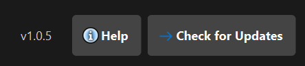
- Help: This button will take you to the page you are currently reading this tutorial
- Check for updates: This button will take you to the github releases page for this app, here you can can compare your version number (within the app) to the newest version shown at the top of the page in github.
Tabs
Visualisation Tab
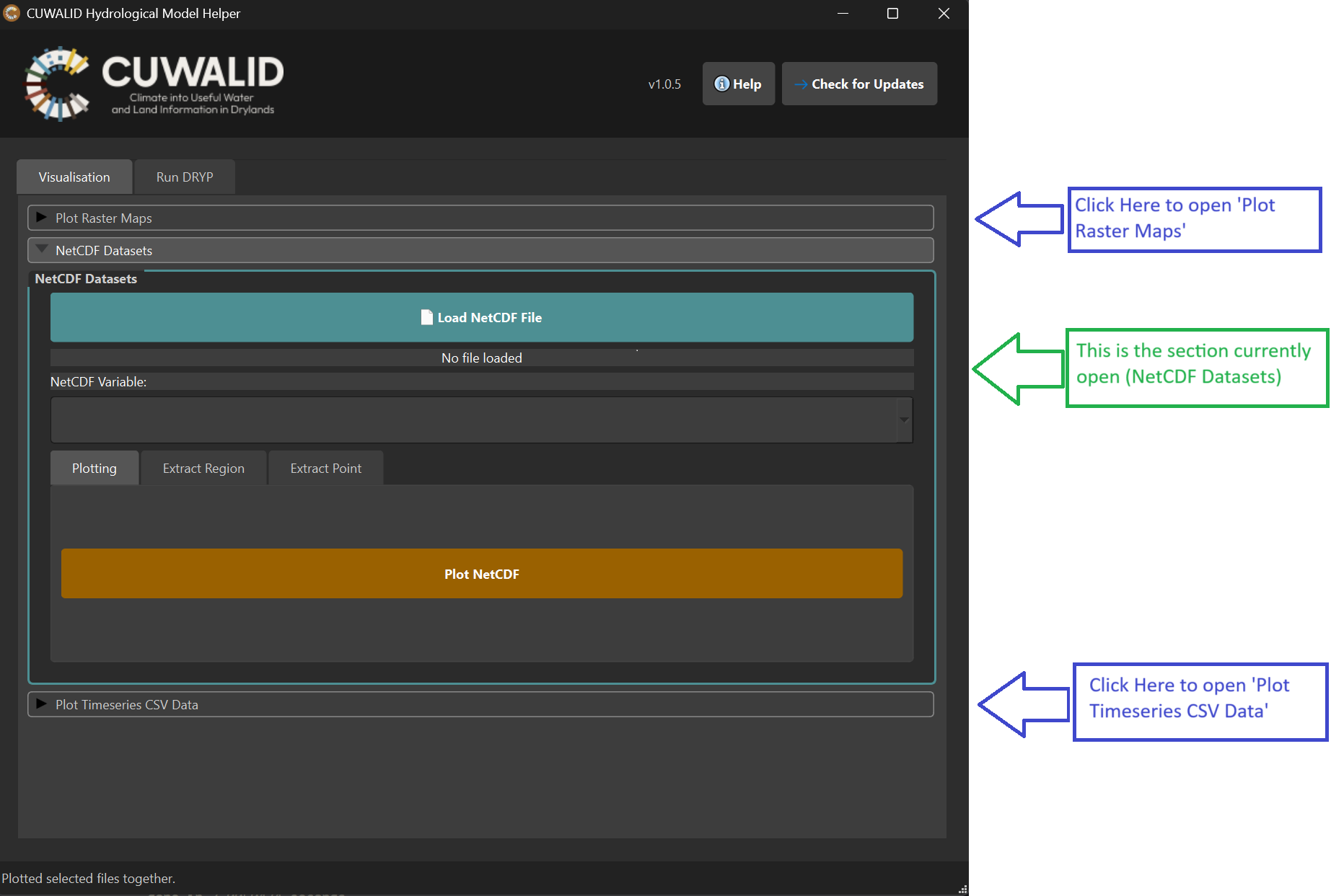
The Visualisation tab allows you to load and visualise different types of data files. This is the tab your program will default to upon opening. The different options are split into dropdown boxes which can be open and closed by clicking on them (only 1 open at a time), these include:
- Plot Raster Maps: This section allows a raster file, shape file and points csv file to be plotted on one figure.
- NetCDF Datasets: Here you can plot both a 2d and 3d (time) NetCDF file, this section also includes functionality to extract data from a region (shape file) or from points (csv file).
- Plot Timeseries CSV Data: The final section provides a place where timeseries csv data can be plotted, for example the csv files that is included within the DRYP model output. Optionally, 2 different files can be uploaded to plot on both the left and right side of the y-axis (useful for different units).
These options are split into sections that you can open by clicking on them as shown in the figure below:
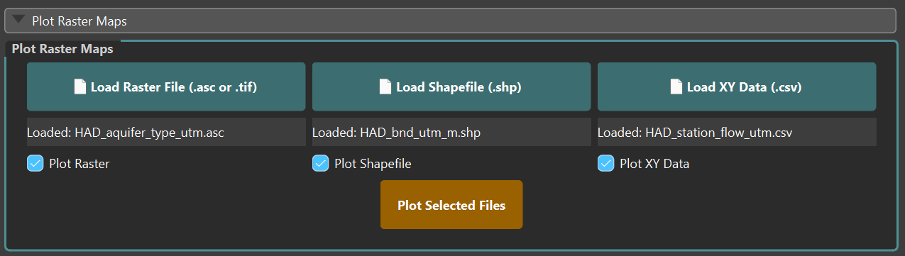
Plot Raster maps
This section of the visualisation tab allows you to plot a combination of raster files (.asc), shape files (.shp) and xy data (.csv) and will allow you to create figures like the following:
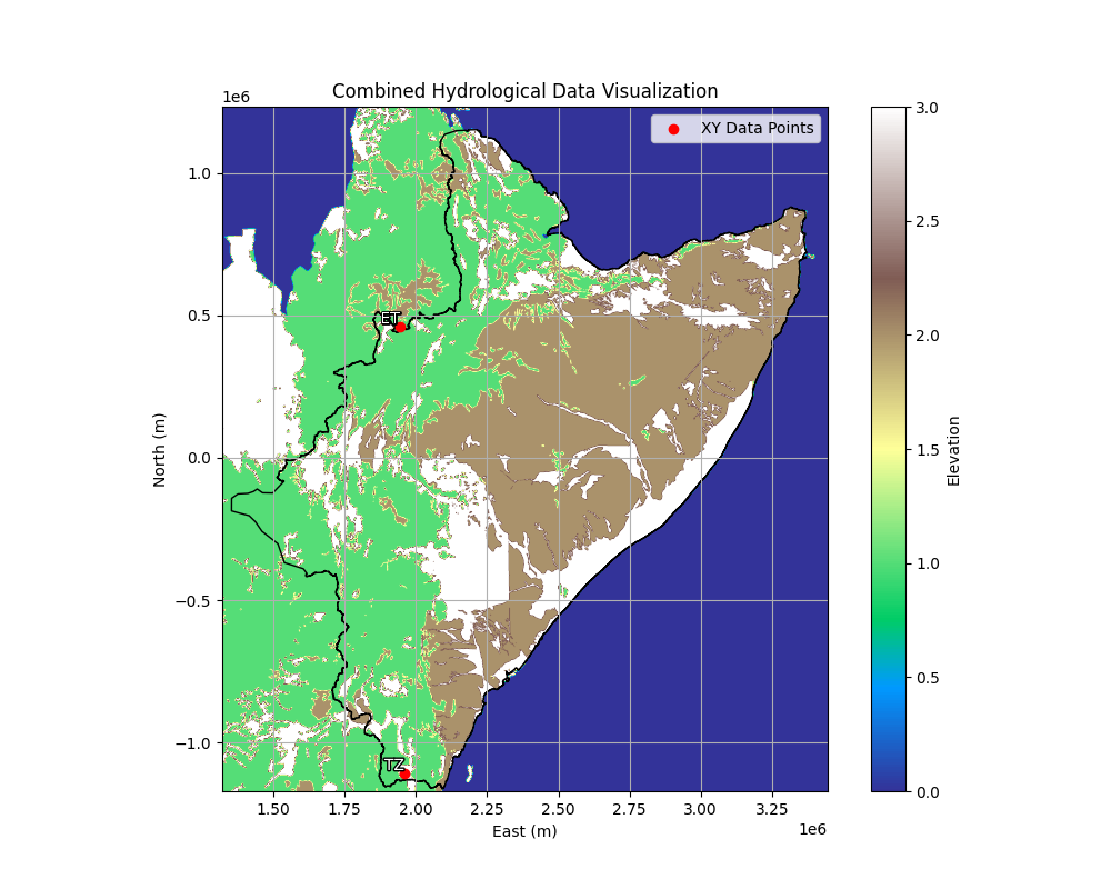
The raster file provides the data shown in colour, the shape file provides the boundry lines and the xy point csv file provides points that are labbelled.
To create these figures you can individually upload each file using the buttons, the labels below give you information on which file has been loaded. The checkboxes allow you to use any combination of the files to create the figure, so it is not necessary to have all the files for this section. Finally the orange plot button will plot these files in a seperate window (using matplotlib).
An example of this section is shown in the figure below:
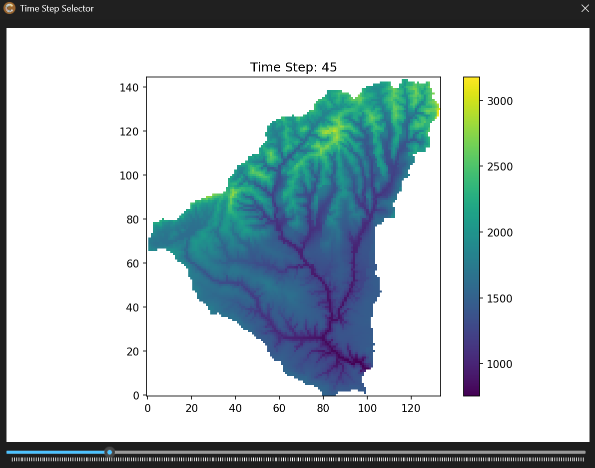
NetCDF Datasets
This section supports plotting of NetCDF files and extracting points or regions from the file to a csv file. The NetCDF can be 2d or 3d with time. If using time, a slider will appear at the bottom of the figure that you can use to slide through the time dimension. An example of this is shown below where you can see the slider at the bottom of the figure in blue:
To use this section you will first want to upload a netcdf file using the button ‘Load NetCDF File’, for large files this may take a minute but your progress is shown in the status bar at the bottom of the app. After this has been uploaded you will see the file name in the label below the button. Below this you can choose which variable from the file you would like to use, this can be chosen by clicking on the drop down and clicking on your choice.
From here you can begin using the 3 features shown as 3 tabs:
- Plotting: This is the default tab where you can immediately plot your selected variable using the orange ‘Plot NetCDF’ button and see the figure as shown above.
- Extract Region: The next tab allows you to use a shape file to extract a region from the netcdf. The first button in this tab (in blue) allows you to upload this shape file, whilst the second will extract the data to a csv file. Upon extracting you will be prompted to save this file and give it a name.
- Extract Point: The final tab allows you to extract specific points from your NetCDF. The blue button allows you to upload a csv file which the rows represent the points and it should have at least 3 columns; ‘North’, ‘East’ and ‘Label’. After uploading this file, the points will appear in the box to the right of the blue button you used for uploading. Here you can select which points you would like to extract, once selected you can use the orange ‘Extract Data’ button to extract the selected points to a new csv file that you will be prompted to name.
Plot Timeseries CSV Data
This final section can help you plot timeseries data from a csv. The section is split into 2 columns, but only one of these is required to start plotting. The second column provides a way to add a second y-axis on the right which is useful if you want to plot data with 2 different units on the same figure.
An example of a figure with 2 y-axis is shown below:
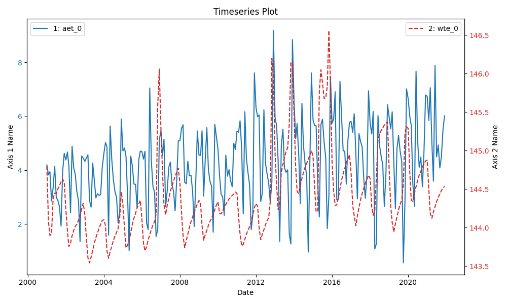
The 2 legends in the top left and rigth corners help you understand the data.
To create this plots you must first upload a csv file (output csv files from DRYP are a great example), which should look similair to this:
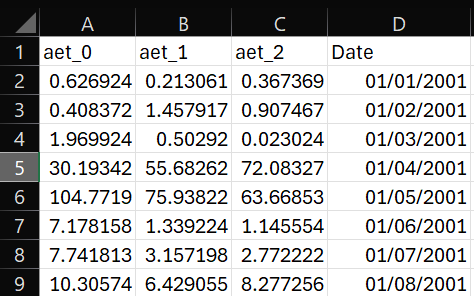
The ‘Date’ column is used for time, but any other column will apear in the grey box below as checkboxes which can be used to select which variables you would like to plot (by default the first 4 are selected).
Below the checkboxes is a text input which is optional and can be used to label the y-axis (useful for giving the units).
Finally the orange ‘Plot Timeseries CSV’ button will plot this data in a new window.
The right column can be used exactly the same way and can even use the same file (useful if you have a csv file with data in different units).
Run DRYP Tab
The Run DRYP tab is where you can run hydrological simulations without needing to write any code. The tab includes 3 buttons:
- Load JSON: The DRYP model uses JSON files to provide the input for the model, this button allows you to upload the confuguration you would like to run (see the input helper for advice on how to create these).
- Input Helper: This button directs you to your browser to the useful CUWALID Input Helper, here you are guided with descriptions on how to create any of the inputs for the CUWALID System (Including DRYP), see the tutorial here.
- Run Model: Click the “Run DRYP” button to execute the hydrological model using the loaded input data.
Below these buttons is a screen with displays the information on how the model is running, if you have experience with coding you will recognise this as the terminal. But if you don’t know coding, don’t worry, this will help provide you information on how the model is running or if it has experienced any issues.
Troubleshooting
If you encounter issues while using the app, check the following:
- Upon crashing errors.txt file may have been created with more information on why it crashed.
- Make sure the files being uploaded meet the required format (sometimes the status bar at the bottom of the app will provide feedback)
- Sometimes your OS System (Windows) may flag the app as harmful, this will prevent it opening and will need to be disabled in your firewall (i.e. Windows Firewall)
If the error can not be solved or you believe this could have been prevented, please use the Github issues page here to inform us. Include the version number (found in the top right corner of your app i.e. ‘v1.0.5’), your OS and version (i.e. Windows 11 Home, Version 24H2) and any information relating to your error. Some of this may be found in a ‘errors.txt’ file where your app file is located on your PC.
Additionally, this is an open-source project so if you are familiar with coding, please feel welcome to fix the error yourself and submit a request to change it through github.